Notes on Artificial Intelligence and Deep Space

2.About the author

David Regordosa is an independent researcher based in Igualada, Catalonia, with a long-standing interest in artificial intelligence and deep-space imaging. His work sits at the intersection of machine learning research and amateur observational astronomy, and is shared through collaborations with non-profit science organisations and academic publications.

He serves as a board member of the Pujalt Observatory (Fundació Ernest Guille i Moliné) and of TIC Anoia, and is a co-founder of TEDx Igualada and Astroanoia.

3.AstropicsLab — AI tools for amateur astrophotography

AstropicsLab (astropicslab.com) is a free, AI-powered web tool that bundles a collection of neural-network models for the enhancement of amateur astrophotography images. Its design goal is not to compete with the established professional pipelines but to make image processing accessible to amateurs who may lack the time or budget to engage with the existing toolchain. The application is in active development; at the time of writing, version 2.0 Beta is the current public release. Tutorials and downloads are available from the project site.

3.1. Processing suite

The current release covers most stages of a typical astrophotography post-processing pipeline:

• AI denoising — multi-noise neural model (see §3.2).
• Star removal and reduction — separates the stellar field from extended structure (see §3.3).
• Object enhancement — sharpens nebular and galactic detail.
• Auto-colourisation — assigns or corrects colour for monochrome and miscalibrated targets.
• 2× super-resolution upscaling.
• Gradient and background removal.
• Auto-stretch with manual levels and curves overrides.
• Luminance-layer separation for independent processing of structure and colour.
• Palette manipulation and three-dimensional rendering effects.
• Star enhancement for the final output.

3.2. Denoising model

A neural network trained on more than 35,000 astronomical images. The model addresses the broad range of noise sources commonly encountered in deep-sky imaging — Gaussian, colour-Gaussian and gradient-Gaussian noise, read and thermal noise, sky-background noise, cosmic-ray events, Poisson noise, speckle noise, and salt-and-pepper noise — by partitioning the input image into 256×256 pixel blocks, processing each block independently, and reassembling the cleaned blocks into the final output. Method details are available in the technical note A denoising pipeline for deep-sky astrophotography.

3.3. Star removal model

This model reduces or removes stars from astronomical images while preserving the fine structural details of nebulae and other deep-sky objects — a common technique used to highlight extended structure that would otherwise be dominated by the stellar field.

The project is named AL in honour of Albert Borràs (1924–2024) — physicist, meteorologist, director of the Pujalt Observatory for sixteen years, co-founder of Astroanoia and Anoiameteo, science communicator, and a great friend, whose insistence on making science accessible to everyone is part of the spirit of this project. Ad astra.

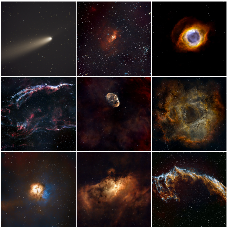
4.Astrophotography

A selection of deep-sky images captured from Igualada, Catalonia. The complete and continuously updated gallery is available on Instagram.

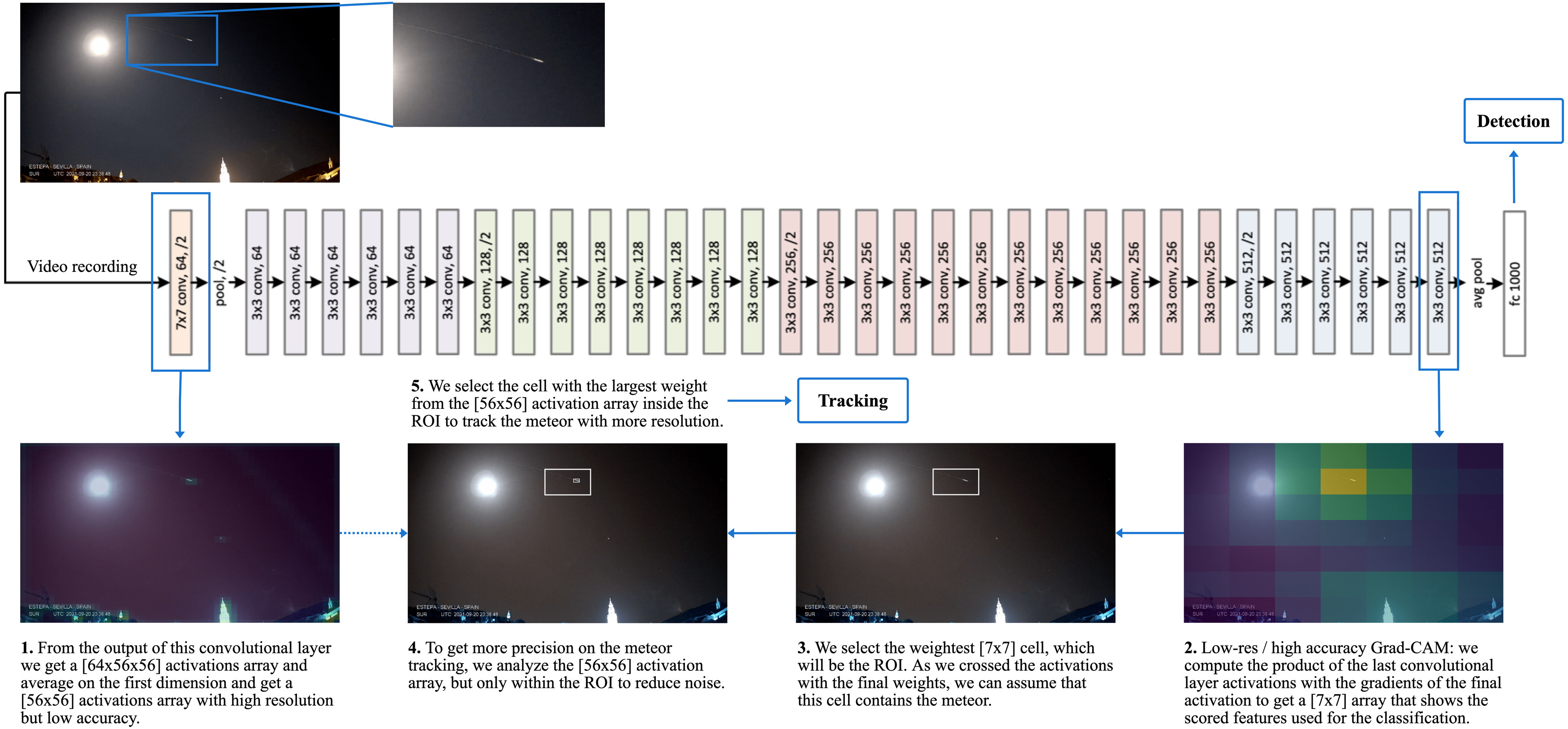
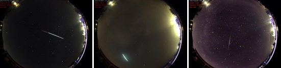
5.Meteor tracking via multi-layer Grad-CAM analysis

This work extends the binary meteor-detection model described in §8 with a localisation procedure that does not require labelled positions. Class Activation Maps (CAM), originally introduced by Zhou et al., identify the spatial regions of an input image that contribute most strongly to a network's classification decision.

We apply Grad-CAM to the final convolutional layer of a ResNet-34 to obtain a coarse Region of Interest (ROI) for the meteor class. We then propagate the ROI to earlier convolutional layers, whose higher spatial resolution refines the localisation; the intersection of the activations at multiple depths yields a precise per-frame meteor position. Iterated frame by frame on a video sequence, the procedure recovers the meteor trajectory.

The method was published in Planetary and Space Science and is also available on arXiv — see §1.

In the visualisation, the blue bounding box corresponds to the ROI extracted from a deep convolutional layer (low spatial resolution, high semantic accuracy), while the red bounding box corresponds to the weighted ROI from an early layer (high spatial resolution). The intersection localises the meteor; iterating across frames yields its trajectory.

The following snippet, adapted from the fast.ai CAM notebook, shows the Grad-CAM extraction at a single layer:

# cls=0 is the meteor class. level=-1 selects the last conv layer of ResNet-34.
cls = 0
level = -1

with HookBwd(learn.model[0][level]) as hookg:
    with Hook(learn.model[0][level]) as hook:
        output = learn.model(x1)
        act = hook.stored
    output[0, cls].backward()
    grad = hookg.stored
w = grad[0].mean(dim=[1, 2], keepdim=True)
cam_map = (w * act[0]).sum(0)

# Normalise weights to [0, 1]: regions of interest in the input image.
avg_acts = torch.div(cam_map, torch.max(cam_map))

# Repeat at level=-5 (first conv layer) for a higher-resolution map,
# then combine the two activations to obtain a precise localisation.
level = -5

Take-away. Combining Grad-CAM activations across layers of a transfer-learned ResNet-34 enables meteor tracking without requiring positional annotations in the training data. Any astronomical observatory in possession of a labelled detection dataset can therefore obtain a tracking system at no additional labelling cost.

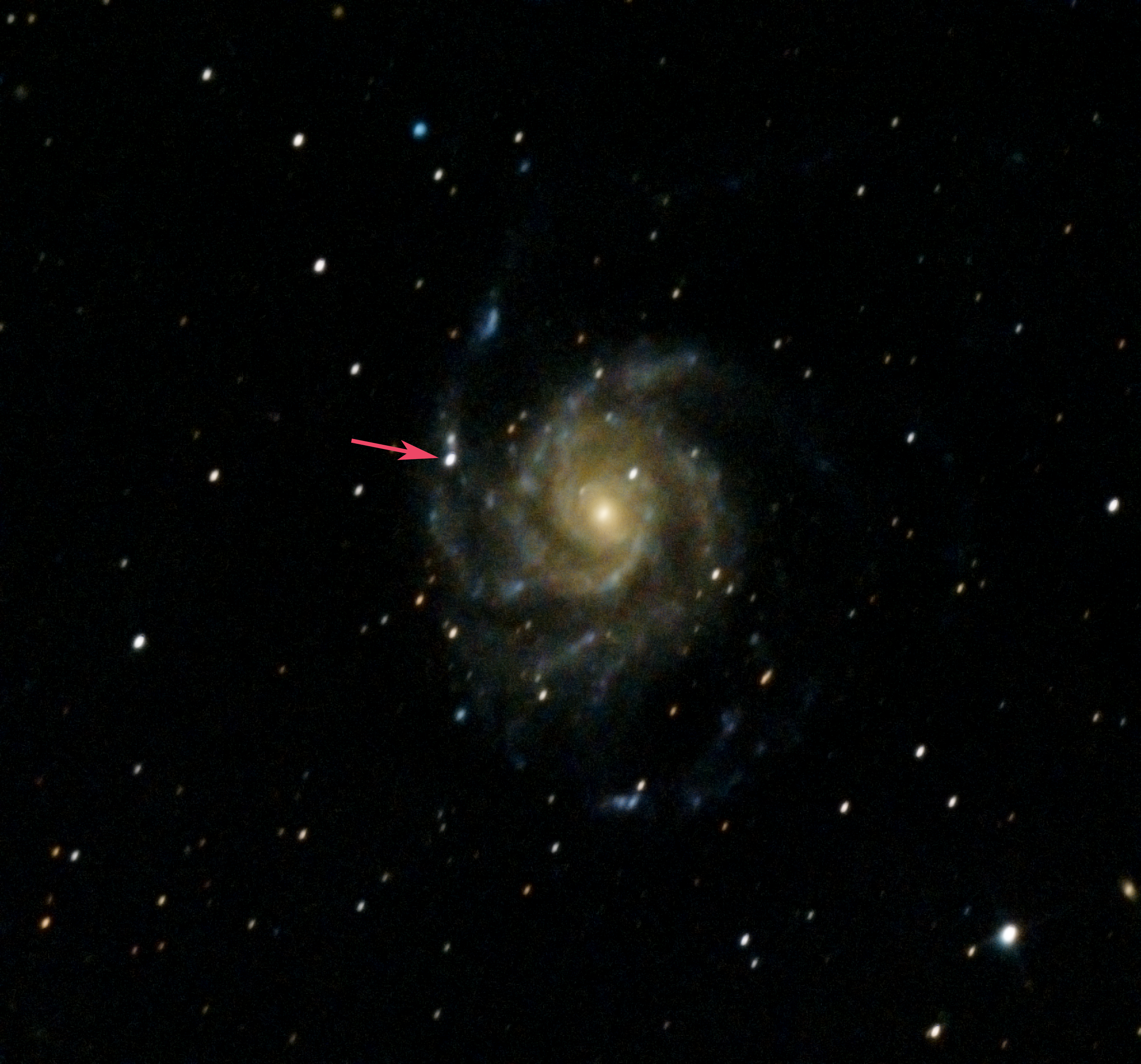
6.The galaxy M101 with supernova SN 2023ixf

An observation of the Pinwheel Galaxy (M101) shortly after the appearance of supernova SN 2023ixf, captured from Igualada.

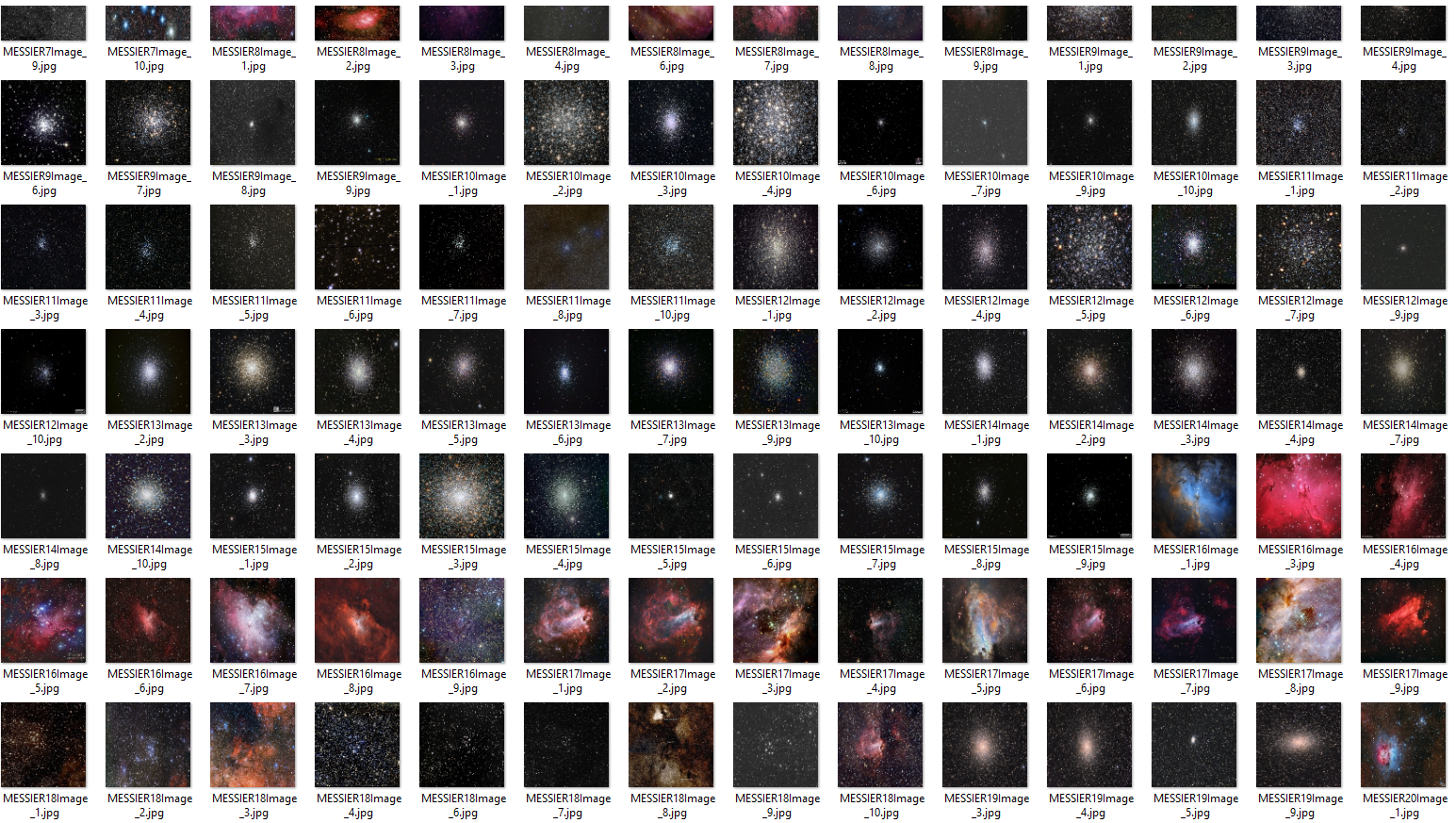
7.BingMeImages — bulk image dataset construction via the Bing API

While building generative models for the colourisation of monochrome deep-space images, we required a large, diverse training set. To that end we developed BingMeImages, a small Python utility for the bulk construction of image datasets from the Bing search API.

The pipeline performs four steps:

1. Query the Bing API for each search term and download the returned images.
2. Consolidate per-query folders into a single output directory.
3. Resize all images to a target resolution.
4. Remove near-duplicates by perceptual hashing.

Querying the full Messier and NGC catalogues yields approximately 3,000 deduplicated images in under one hour.

# Build the query list for the Messier and NGC catalogues.
my_objects = []
for num in range(1, 111):
    my_objects.append('MESSIER ' + str(num))
for num in range(1, 7840):
    my_objects.append('NGC ' + str(num) + ' space')

# Run the full pipeline:
#   my_objects : list of queries
#   200        : images to download per query
#   ./ufo      : output directory
#   160        : resize target (160 x 160 pixels)
createDataset(my_objects, 200, "./ufo", 160)

Source code: github.com/pisukeman/bingMeImages.

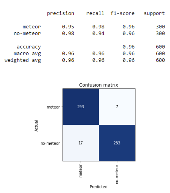
8.Meteor detection via transfer learning on ResNet-34

A binary classifier for the automatic detection of meteors in still images and video frames. The model is trained on 57,000 frames captured by the AlphaSky all-sky camera at the Pujalt Observatory, using transfer learning on a ResNet-34 backbone pretrained on ImageNet, and built with the fast.ai framework.

The dataset is strongly imbalanced — non-meteor frames vastly outnumber meteor frames — and the imbalance is mitigated through aggressive data augmentation rather than resampling, which preserves the natural distribution of negatives at training time.

On the held-out test set the model achieves a recall of 0.98 at the meteor class. The trained weights are released as guAIta_latest_version.pkl.

Inference is straightforward; the environment is provided as an Anaconda YAML:

learn = load_learner("guAIta_latest_version.pkl")
predict = learn.predict(image)
if predict[0] == "meteor" and predict[2][0] > scoring:
    # meteor captured

The full methodology is documented in the corresponding Master's dissertation (in Spanish): Meteor detection with deep learning.

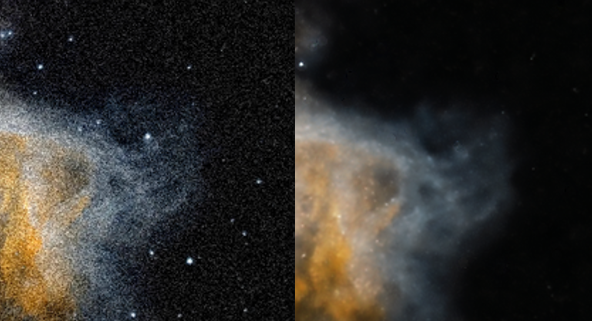
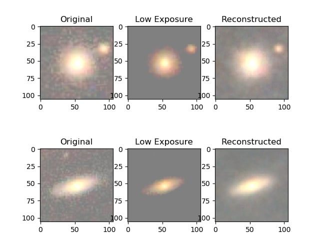
9.Restoring exposure in galaxy images with autoencoders

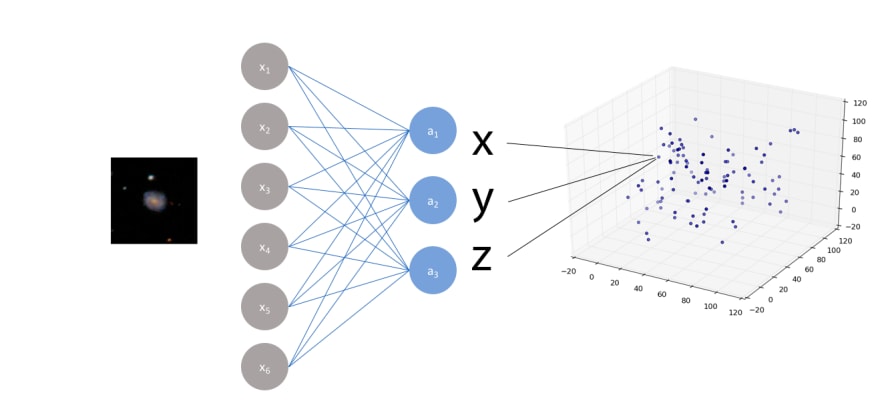
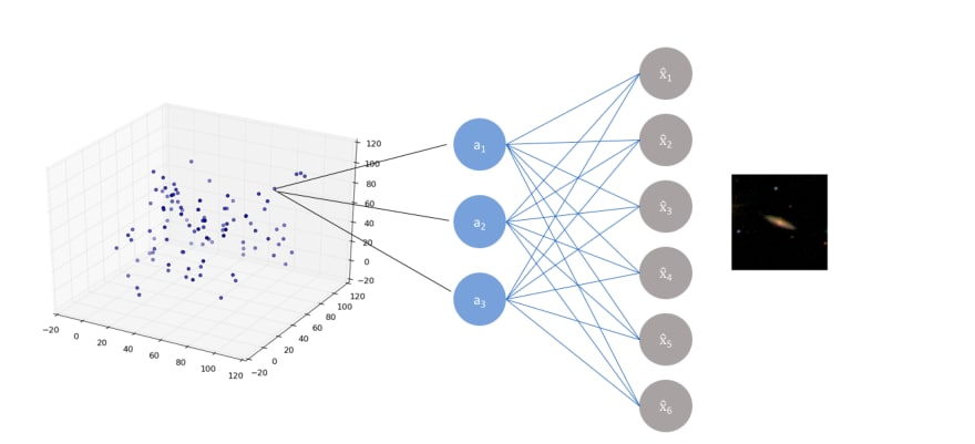
Autoencoders are neural networks with a constrained topology — input layer, smaller "bottleneck" hidden layer, and output layer of the same size as the input — designed to learn compressed, denoised data representations in an unsupervised manner.

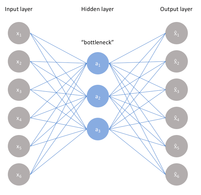
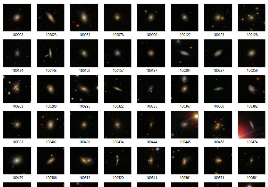
We train an autoencoder on galaxy images from the Galaxy Zoo dataset on the Zooniverse platform (61,000 images at 106×106 pixels) and split the trained network into its encoder (input → latent code) and decoder (latent code → reconstruction) components.

The key training trick is asymmetric input/output pairing: low-exposure (synthetically attenuated) images are presented as inputs while their original counterparts are presented as targets. The network therefore learns a mapping from underexposed to fully-exposed images.

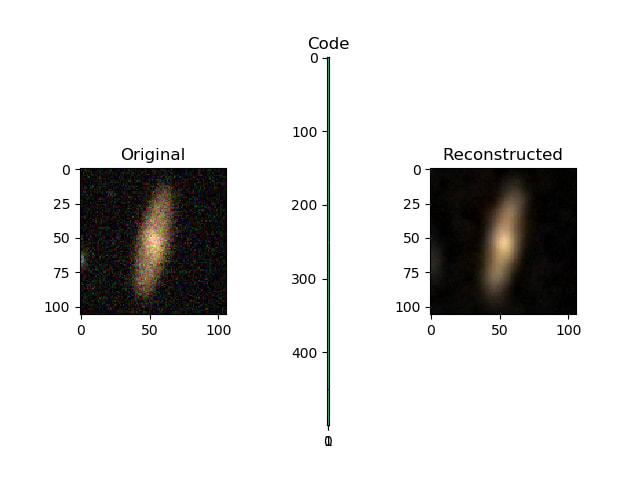
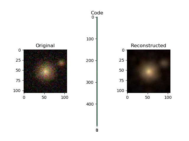
The simulation of low exposure is implemented as a per-pixel attenuation:

x_train, x_test = train_test_split(x_train, test_size=0.1, random_state=42)
x_train_noise = simulate_low_exposure(x_train)
x_test_noise  = simulate_low_exposure(x_test)

def simulate_low_exposure(x, max, min, perc):
    return np.where(x - perc > min, x - perc, min)

Training the autoencoder:

def build_one_layer_autoencoder(img_shape, code_size):
    # Encoder.
    encoder = Sequential()
    encoder.add(InputLayer(img_shape))
    encoder.add(Flatten())
    encoder.add(Dense(code_size))

    # Decoder.
    decoder = Sequential()
    decoder.add(InputLayer((code_size,)))
    decoder.add(Dense(np.prod(img_shape)))
    decoder.add(Reshape(img_shape))

    return encoder, decoder

# 1,000-dimensional bottleneck.
encoder, decoder = build_one_layer_autoencoder(IMG_SHAPE, 1000)
inp_shape = Input(IMG_SHAPE)
code = encoder(inp_shape)
reconstruction = decoder(code)
autoencoder = Model(inp, reconstruction)
autoencoder.compile(optimizer='adamax', loss='mse')

# Train: low-exposure inputs, original targets.
history = autoencoder.fit(
    x=x_train_noise, y=x_train,
    epochs=10,
    validation_data=[x_test_noise, x_test],
)

An earlier version of this work appeared on dev.to.